3D Crack Growth Abaqus XFEM Simulation – Full Step-by-Step Guide

Simulating 3D crack growth Abaqus XFEM simulation is one of the most powerful (and often misunderstood) techniques in fracture mechanics. If you’ve ever attempted it and failed—or didn’t know where to begin—this guide is for you. Simulating fracture is one of the most misunderstood parts of finite element analysis. Many tutorials are incomplete, and most don’t explain critical settings like PHILSM, PSILSM, or Status XFEM.

In this post (and the full video tutorial), you’ll walk through the entire setup for a 3D XFEM crack growth simulation in Abaqus:

• Geometry and crack modeling
• Material properties with damage
• XFEM interaction settings
• Boundary conditions and loading
• Mesh setup and output fields
• Postprocessing with crack front fields

🎥 Watch the full tutorial here:

Starting with Geometry: Modeling Plate and Crack

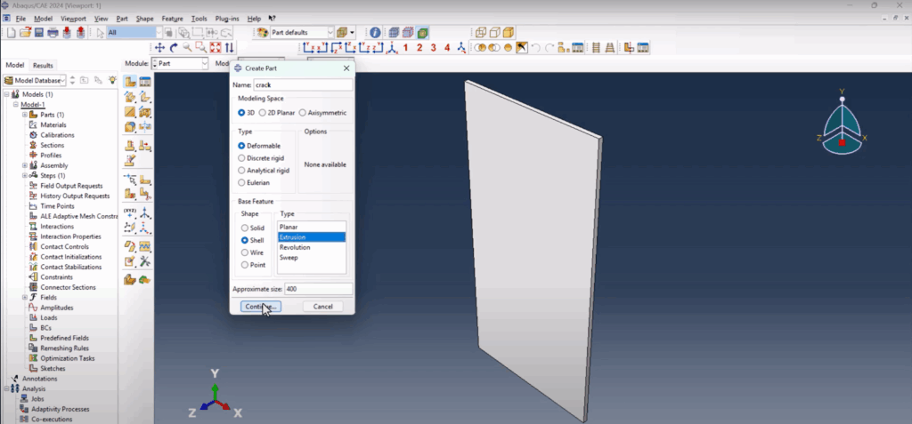
We begin by creating two parts:

1. Plate
   • Type: 3D deformable solid
   • Dimensions: 100 mm × 200 mm × 3 mm (extruded depth)
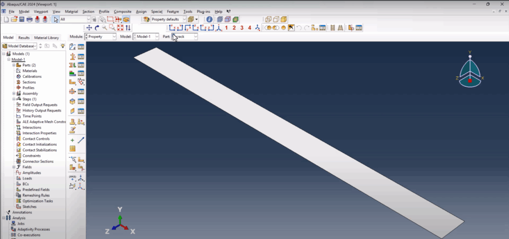
2. Crack
   • Type: 3D deformable shell
   • Geometry: A simple 40 mm line representing the initial crack front
   • Extrusion depth: 3 mm (same as plate thickness)

It’s important to model the crack as a separate 3D surface—not just a line. XFEM requires an actual crack face in 3D to compute enrichment functions correctly. This is one key difference from 2D XFEM setups.

Material Properties (Aluminum XFEM Pack)

To keep things realistic, we use aluminum as the base material and define:

• Elastic modulus and Poisson’s ratio
• Plasticity (since crack tips undergo yielding)
• Damage Initiation: Maximum Principal Stress = 350 MPa
• Damage Evolution: Fracture energy method (input as energy per area)

📦 You can download these ready-made properties from FEAMaster Material Packs. It’s a free resource made to simplify simulation setup.

After defining the material, we assign it to a solid homogeneous section and apply it to the plate.

Assembly & Crack Alignment

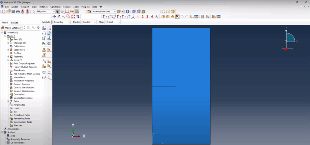
In the Assembly module:

• We position the crack object such that it intersects the center of the plate.
• Abaqus requires the crack surface and the cracked body to be spatially connected.
• Use Translate to align the crack with the plate accurately—typically along the mid-plane.

This ensures the crack grows in a realistic, physical manner.

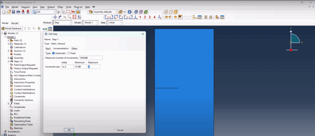
Step Definition & Output Controls

We define a Static General Step and activate nonlinear geometry (NLGEOM).

Step settings:

• Total time: 1
• Initial increment: 1e-2
• Minimum increment: 1e-9
• Maximum increment: 1

Then go to the Field Output Manager and enable critical fracture fields:

• PHILSM (Level set field)
• PSILSM (Crack direction)
• Status XFEM (Enrichment status of elements)

These outputs are essential for visualizing crack growth and interpreting XFEM behavior.

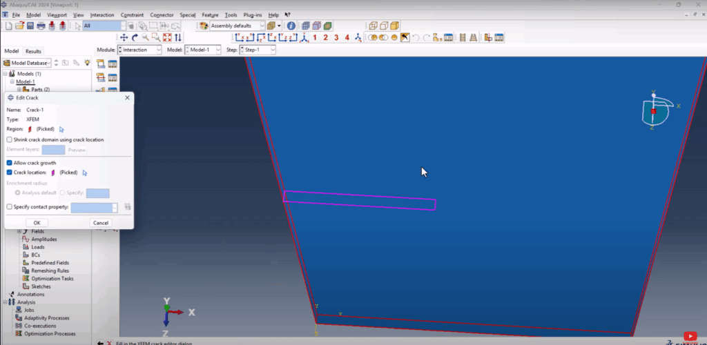
XFEM Interaction Setup

1. Crack Interaction
   • Go to Special > Crack > Create
   • Type: XFEM
   • Assign the plate as the crack domain
   • Assign the crack surface as the initial crack location
   • The crack turns magenta when assigned correctly
2. XFEM Crack Growth
   • Create another interaction (Step: Initial)
   • Assign the same crack name
   • This enables the automatic growth of the crack based on field values

After this step, you’ll see small “X” marks on the part—these indicate XFEM enrichment is active.

Boundary Conditions & Load Application

We apply two boundary conditions:

1. Fixed (Encastre)
   • Assigned to the bottom face of the plate
   • Prevents all movement and rotation
2. Displacement (Y direction only)
   • Applied to the top surface
   • Allows vertical displacement only
   • Restricts X and Z translations

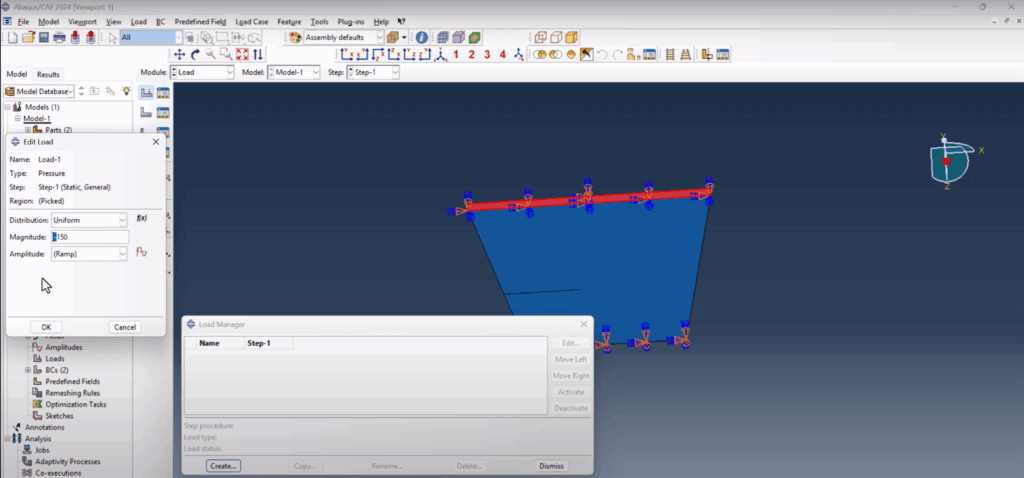
Then we apply a tensile load:

• Type: Surface Pressure
• Magnitude: Negative (e.g., -1 MPa) to simulate tension
• Surface: Top face of the plate

This loading mode mimics Mode I crack opening (pure tensile crack growth).

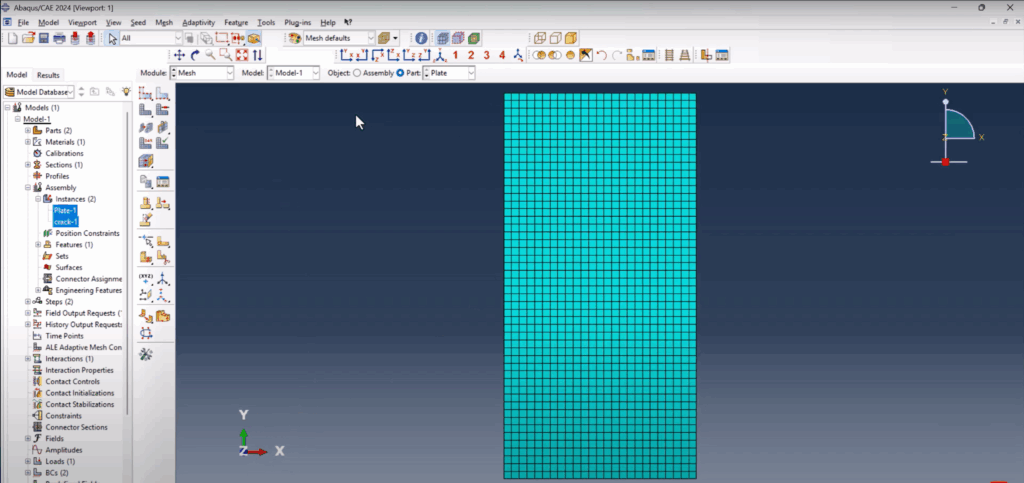
Mesh Settings

We refine the mesh only where needed:

• Plate mesh seed: 4 mm
• Crack part: not meshed, as XFEM handles enrichment internally
• Mesh type: C3D8 (8-node bricks)

Important: The crack part should remain as a shell with no section assigned. Abaqus will ignore it as geometry but still use it to define enrichment.

Job Setup and Execution

Create a job named XFEM_Crack_Growth_3D and assign:

• The full model
• Default memory and parallel settings
• Submit and monitor

If you receive a warning about missing sections for some parts (like the crack), you can safely ignore it. Abaqus will proceed using the enriched crack domain settings.

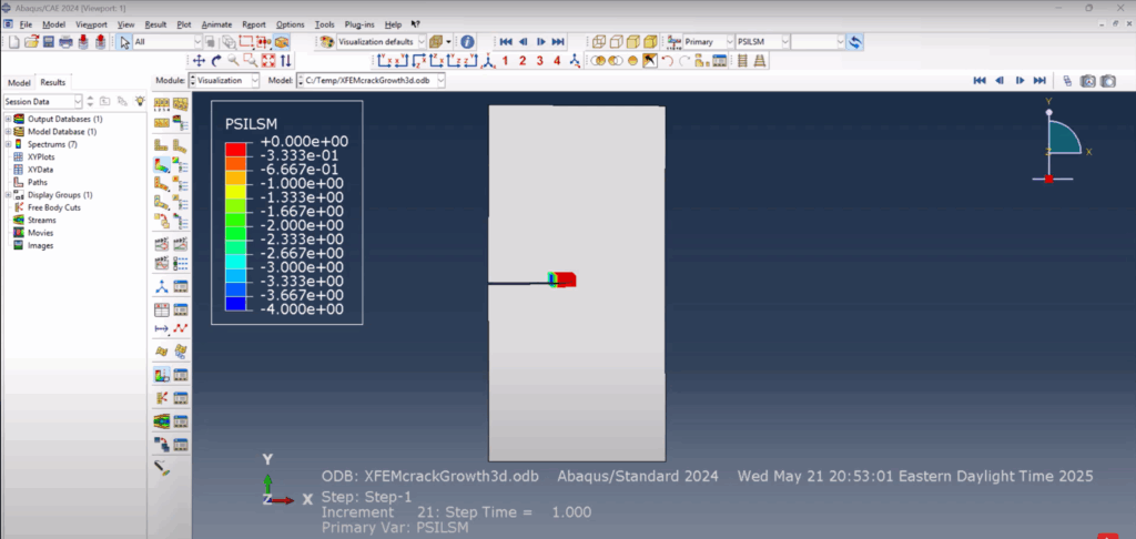
Results and Crack Growth Visualization

Once the job is completed:

1. Enable Feature Edges in Visualization settings
2. Animate the results to see the crack propagation over time
3. Toggle PHILSM and PSILSM:
   • PHILSM represents the distance from the crack surface
     • 0: crack surface
     • < 0: inside the crack
     • 0: uncracked material
   • PSILSM shows the crack front direction
     • It starts at 0 and grows outward as the crack advances
4. Plot Status XFEM to see which elements are enriched (1 = cracked)
5. Visualize Displacement Field (U2) to confirm crack opening behavior

Together, these tools give you a full understanding of how the crack initiated, how far it propagated, and how the material responded.

3D Crack Growth Abaqus XFEM Simulation

Why This 3D Crack Growth Abaqus XFEM Simulation Matters

Most XFEM tutorials focus on 2D models or skip the enrichment logic. This example gives you:

• ✅ A full 3D setup with realistic aluminum properties
• ✅ Proper fracture and damage mechanics
• ✅ Clear explanation of PHILSM and PSILSM
• ✅ Postprocessing that shows actual growth direction

Whether you’re modeling brittle failure, fatigue pre-cracks, or fracture toughness, this workflow applies to all.

Download the Files and Skip the Setup

🎯 Want to skip the setup and get straight to results?

Download the full model, XFEM material properties, and ready-to-run .cae file:

👉 Download the XFEM Crack Growth 3D Simulation Files

Conclusion

Simulating 3D crack growth in Abaqus with XFEM isn’t just about clicking checkboxes—it requires a clear understanding of enrichment, crack location, mesh strategy, and output interpretation. But once you set it up right, the results are powerful.

Now you have a full blueprint. You can modify this setup for other materials, different crack shapes, or loading conditions like bending or mixed mode.

📺 Watch the full video tutorial now:
👉 3D Crack Growth XFEM in Abaqus – YouTube

💬 Questions? Leave a comment or message me on LinkedIn. Your feedback helps improve future tutorials.

🔔 Subscribe to FEA Master for more detailed guides on welding, fracture, fatigue, and everything Abaqus.