Abaqus DFLUX Welding Simulation has always been a hot topic! If you’ve ever searched for a clear, complete guide to running an Abaqus DFLUX welding simulation, chances are you were disappointed. Most tutorials either skip the critical steps or hide the actual code.
That’s why I created this walkthrough.
This is the only video you need if you want to run a welding simulation in Abaqus using a moving heat source and a custom DFLUX subroutine. We’re building the model from scratch, writing the code step by step, and simulating the weld—no guesswork, no missing pieces.
And yes, you get the full DFLUX code.
🎥 Watch the full tutorial now:
👉
Sponsored by HeatShape – Cloud-Based Welding Simulation
Before we dive in, a quick thank you to HeatShape for sponsoring this video.
HeatShape is a browser-based simulation platform built for welding and additive manufacturing. No software installation, no Fortran, no subroutines—just define your weld, choose your process, and simulate directly in your browser.
If you’re tired of debugging DFLUX routines and want an easier way to simulate welding, this platform is for you.
👉 Try HeatShape now — free demo available
Step-by-Step Abaqus DFLUX Welding Simulation Setup
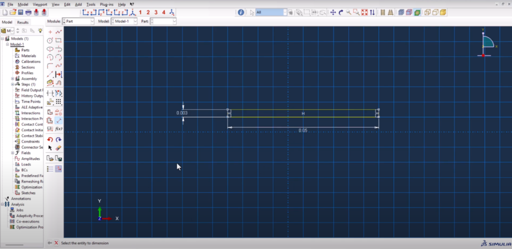
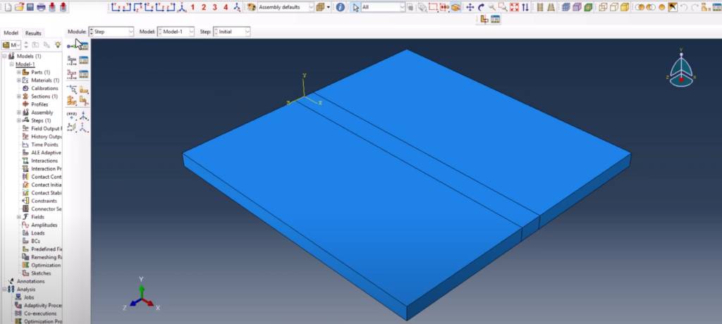
We start by creating a 3D deformable solid part and sketching a simple rectangle—0.025m by 0.050m. After extrusion, we partition the model to refine the mesh where the flux will move. This is critical for capturing accurate temperature gradients in your Abaqus DFLUX welding simulation.
Material Properties
We define temperature-dependent properties for:
- Density
- Thermal conductivity
- Specific heat
Values are copied from an Excel file. You can get the full material property set from femaster.com. Once defined, the section is assigned to the part.
To simplify heat source definition, we translate the part so that the origin (0,0) aligns with the starting point of the weld path. This makes coding the moving heat source much easier.
Assembly & Translation
To simplify heat source definition, we translate the part so that the origin (0,0) aligns with the starting point of the weld path. This makes coding the moving heat source much easier.
look at the XYZ datum. It is the starting point of the flux
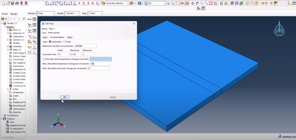
Step Definition and Output Controls
We create a Heat Transfer Step with a total time of 25 seconds and appropriate time increment settings. Field outputs are simplified to only include nodal temperature, reducing the file size and focusing on relevant results.
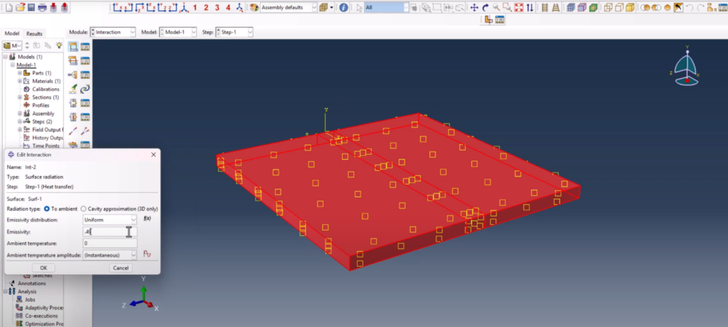
Interactions: Surface Film and Radiation
We define two interactions to simulate heat loss:
- Surface Film Condition with realistic convection properties
- Surface Radiation using an emissivity of 0.49 and ambient temperature of 25°C
These steps ensure a realistic cooling model during the simulation.
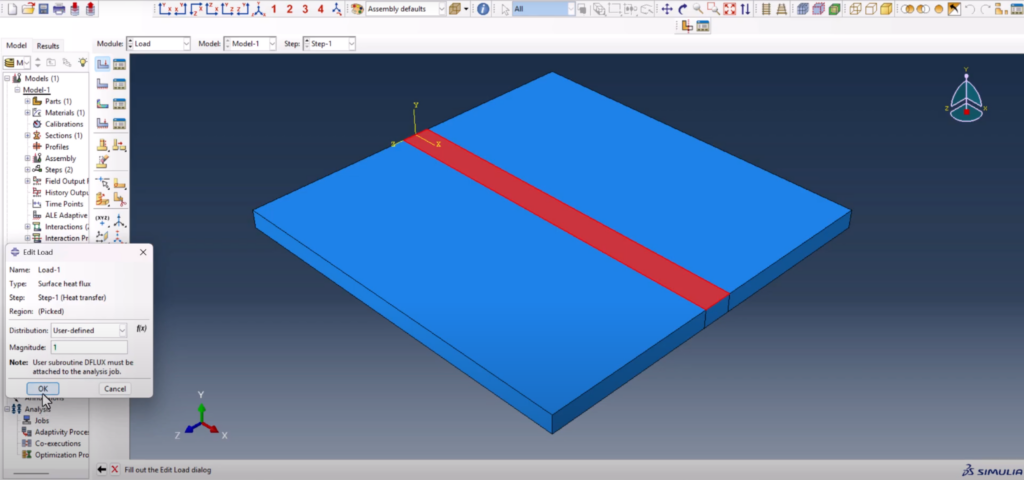
Applying the Heat Load
We create a Surface Heat Flux load using the User Defined option. This tells Abaqus to expect a custom DFLUX subroutine. We also apply a Predefined Field to set the initial temperature at 25°C across the entire model.
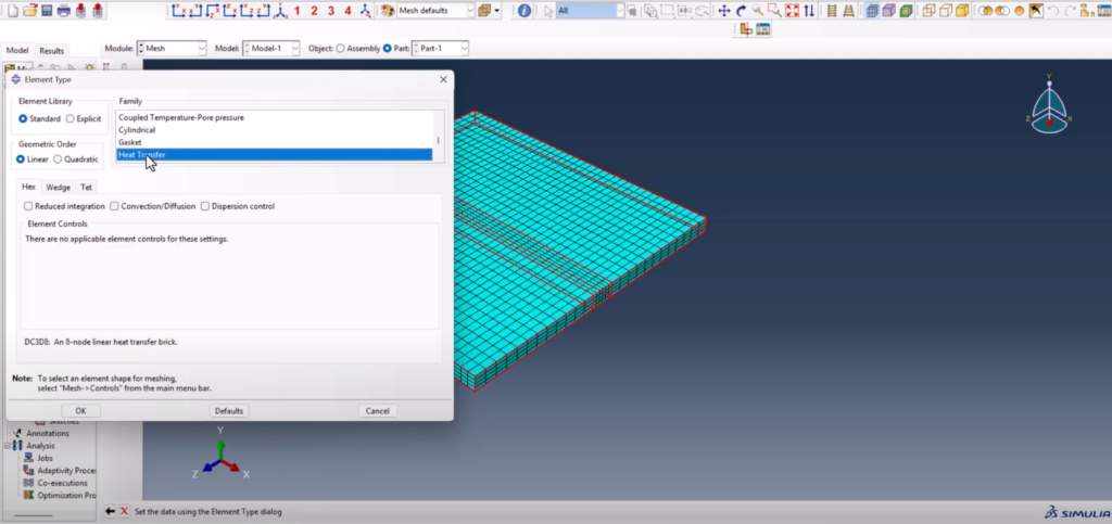
Meshing and Element Assignment
The mesh is refined in the weld zone, using:
- 40 elements across the partitioned lines
- 6 elements in constrained edges
- 4 elements in the remaining parallel lines
We assign heat transfer elements (DC3D8) to the part before running the job.
Writing the DFLUX Subroutine
The subroutine is written in Intel Fortran using Visual Studio. We open the Abaqus documentation, locate the DFLUX template, and paste it into our Fortran project.
Here’s what the code does:
- Defines a moving Gaussian heat source
- Moves in the X direction at a given speed
V - Applies flux only within a cutoff radius
R0using a bell-shaped (Gaussian) decay - Uses
FLUX(1)to apply temperature load at each integration point
This is a fully working Abaqus DFLUX welding simulation code—transparent, tested, and explained.
      SUBROUTINE DFLUX(FLUX,SOL,KSTEP,KINC,TIME,NOEL,NPT,COORDS,
     1 JLTYP,TEMP,PRESS,SNAME)

      INCLUDE 'ABA_PARAM.INC'

      DIMENSION FLUX(2), TIME(2), COORDS(3)
      CHARACTER*80 SNAME

C --- Coordinates and time
      X = COORDS(1)
      Y = COORDS(2)
      Z = COORDS(3)
      T = TIME(2)

C --- Heat source parameters
      X0 = 0.0
      Z0 = 0.0
      V  = 0.003       ! m/s (torch speed)
      Q  = 400.0       ! W (total input power)
      RO = 0.0025      ! m (effective radius)
      PI = 3.141593

C --- Moving heat center
      XC = X0 + V*T
      ZC = Z0

C --- Gaussian surface heat flux (in W/m²)
      RO2 = RO**2
      DIST2 = (X - XC)**2 + (Z - ZC)**2
      Q0 = (3.0 * Q) / (PI * RO2) * EXP(-3.0 * DIST2 / RO2)

      FLUX(1) = 0.0
      IF (DIST2 .LT. RO2) THEN
         FLUX(1) = Q0
      ENDIF

      FLUX(2) = 0.0

      RETURN
      END
Final Steps: Running and Validating the Job
Before submission, we update model attributes with:
- Stefan-Boltzmann constant
- Absolute zero temperature (-273.15°C)
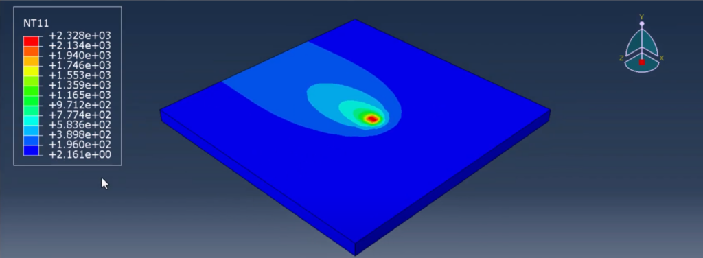
We then assign the DFLUX file and run the job. Once completed, we view the contour plot and animation, showing the smooth movement of the heat source and a peak temperature of ~2600°C.
If the mesh were finer, the animation would be even smoother—but the temperature field and behavior are already realistic and useful.
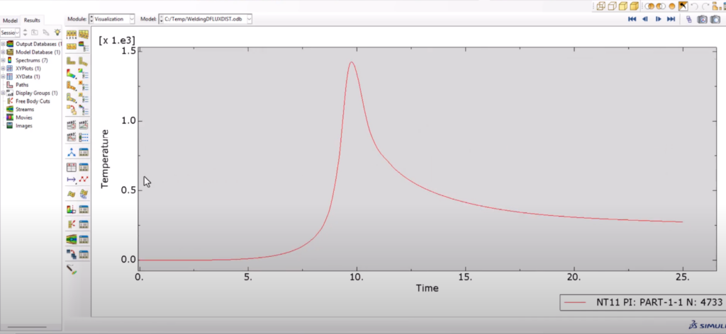
Postprocessing: Extracting Nodal Temperature
In the XY Data Manager, we extract temperature versus time data from a selected node. This helps verify that the heat flux input behaves as expected, and that the simulation captures the thermal response accurately.
Why This Abaqus DFLUX Welding Simulation Matters
This tutorial isn’t just a demonstration. It’s a full teaching tool for anyone wanting to simulate welding processes in Abaqus using their own subroutines.
Whether you’re a student, researcher, or industry engineer, this method gives you:
- Full control over heat source definition
- A solid understanding of thermal simulation flow
- A ready-made DFLUX subroutine that you can modify and reuse
Download the Files or Skip the Setup
🎯 Want to skip the full model setup and jump straight into your Abaqus DFLUX welding simulation?
You can download the complete simulation package—including the .cae file, .inp file, and full DFLUX subroutine—for immediate use in your own analysis.
👉 Download the Abaqus DFLUX Welding Simulation Package
Whether you’re a student, researcher, or professional engineer, this ready-to-run package saves hours of setup and lets you focus on the results.
Conclusion
With this video and blog, you now have everything you need to perform an Abaqus DFLUX welding simulation from scratch. From model setup to writing the code, assigning loads, running the job, and extracting results—it’s all here.
✅ No skipped steps
✅ No hidden code
✅ Real-world-ready simulation workflow
📺 Watch the full video now and follow along step by step:
👉 Abaqus DFLUX Welding Simulation – The Only Tutorial You Need
💬 Found it helpful? Leave a comment on YouTube or let me know on LinkedIn. Your feedback helps me grow and keeps this content coming.
🔔 Subscribe to FEA Master for more tutorials like this!
