Abaqus Goldak DFLUX Welding Simulation – Full Tutorial With Code

If you’ve ever struggled to simulate realistic welding in Abaqus—especially using the Goldak double ellipsoid heat source—you’re not alone. Most tutorials skip critical steps or hide the actual subroutine code.

This post walks you through the entire Abaqus Goldak DFLUX welding simulation, step by step. From building the model and writing the subroutine, to applying body heat flux and validating the results—nothing is skipped.

And yes, you get the full DFLUX code and downloadable files.

🎥 Watch the full video tutorial:

Why Use the Goldak Model in Abaqus?

The Goldak double ellipsoid heat source is widely used in welding simulation because it provides a more realistic representation of heat distribution during arc welding. It divides the heat input into front and rear quadrants using two 3D ellipsoids, offering excellent control over penetration and bead shape.

In this tutorial, you’ll learn how to implement Goldak’s model using the DFLUX subroutine in Abaqus.

Step-by-Step Guide to the Abaqus Goldak DFLUX Welding Simulation

1. Create the Geometry and Partition for Mesh Refinement

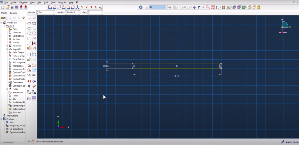
We start by creating a 3D deformable solid part using a rectangular sketch. The dimensions are 0.025 m in width and 0.050 m in height. Once extruded, this creates a solid block where we will later apply the moving heat source.

To ensure accurate thermal gradients in the weld zone, we partition the geometry. Two vertical sketch lines are added to the face of the part, concentrating the mesh where the heat flux will move. This step is crucial—not only does it localize computational effort, but it also improves gradient resolution in the region of interest.

2. Assign Temperature-Dependent Material Properties

We define:

• Density
• Thermal conductivity
• Specific heat

All properties are temperature-dependent. You can grab the ready-to-use Excel sheet from the FEAMaster Material Properties Package for free.

3.Assembly & Translation

The part is assembled and then translated so the bottom-left corner lies at the global origin (0, 0, 0). This small adjustment makes a big difference: it simplifies how we define the position of the moving heat source in the DFLUX subroutine. By aligning the heat source with (X0, Z0) = (0, 0), we make the movement equation XC = X0 + V*T easy to control and verify.

This also guarantees the model’s coordinate system matches our subroutine logic.

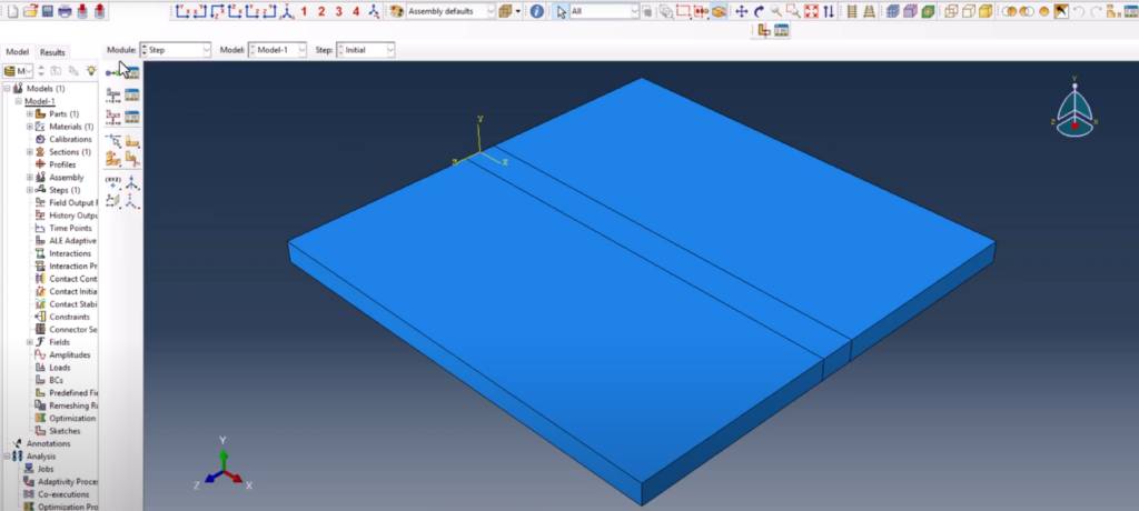
look at the XYZ datum. It is the starting point of the flux

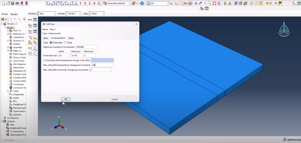
4. Set Up Heat Transfer Step

A Heat Transfer step is created following the initial step. This transient step will control the simulation over time.

• Time period: 25 seconds
• Time increment range: minimum 1e-10, maximum 1
• Total time steps: sufficient for smooth movement of the heat source

In the Field Output settings, we remove all unnecessary output variables and retain only nodal temperature (NT). This reduces file size and improves postprocessing speed.

5. Define Heat Loss Interactions

Two types of interactions are defined to represent environmental heat loss:

1. Surface Film Condition
   • Assigned to the top face
   • A realistic convection coefficient is added
   • Sink temperature is 25°C to simulate ambient conditions
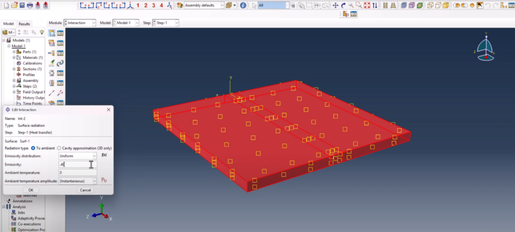
2. Surface Radiation
   • Applied to the same face
   • Emissivity is set to 0.49
   • Ambient temperature = 25°C

These combined interactions allow the model to realistically cool as it’s heated by the moving heat source—mimicking real-world welding conditions.

6.Meshing and Element Assignment

The mesh plays a crucial role in thermal simulations. We define a non-uniform structured mesh:

• 40 elements across the center weld path
• 6 elements near constrained boundary edges
• 4 elements in surrounding directions

The element type is switched to DC3D8—a 3D linear brick element suited for transient heat transfer problems.

Even though the initial mesh is coarse, it balances simulation time and accuracy. For more detailed studies, especially metallurgical predictions, further refinement is recommended in the weld zone.

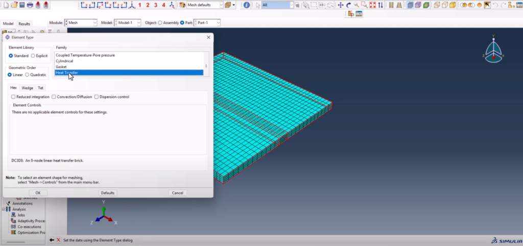
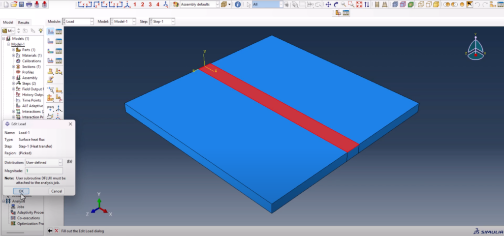
7. Apply the Body Heat Flux Using DFLUX

We apply a Surface Heat Flux load using the User Defined option. This tells Abaqus to use the custom subroutine (DFLUX) to determine the magnitude and distribution of the heat input.

• Surface is selected manually
• “User-defined” is chosen as the load type
• Magnitude is set to 1 (the subroutine will override this)

We also define a Predefined Field for temperature: the model begins uniformly at 25°C. This baseline ensures that temperature increases during the simulation are driven entirely by the moving heat input.

Writing the Goldak DFLUX Subroutine

The subroutine is written in Intel Fortran using Visual Studio. We start by copying the official DFLUX template from the Abaqus documentation, then insert custom logic to define a Gaussian moving heat source.

Key features of the subroutine:

FLUX(1) controls the heat applied at each point; FLUX(2) is left at zero

The heat center moves in the X direction over time using XC = X0 + V*T

A bell-curve distribution is created using exp(-3 * DIST2 / R0^2)

Heat is applied only inside the effective radius, reducing computation time

      SUBROUTINE DFLUX(FLUX,SOL,KSTEP,KINC,TIME,NOEL,NPT,COORDS,
     1 JLTYP,TEMP,PRESS,SNAME)
C
      INCLUDE 'ABA_PARAM.INC'
      DIMENSION FLUX(2), TIME(2), COORDS(3)
      CHARACTER*80 SNAME

C     Coordinates
      X = COORDS(1)
      Y = COORDS(2)
      Z = COORDS(3)

C     Heat source center (moving in X with time)
      XC = 0.0 + 0.002 * TIME(2)
      YC = 0.0D0
      ZC = 0.0D0

C     Goldak parameters (in meters)
      a  = 6  / 1000.0
      c  = 5  / 1000.0
      bf = 3.46 / 1000.0
      br = 8 / 1000.0
      ff = 0.57D0
      fr = 1.43D0
      PI = 3.1415D0

C     Heat input parameters
      eta = 0.8
      V   = 23.0
      I   = 232.0
      Q   = eta * V * I

      Qr = (6.0D0 * Q * fr) / (a * br * c * PI * SQRT(PI))
      Qf = (6.0D0 * Q * ff) / (a * bf * c * PI * SQRT(PI))

C     Rear half (X <= XC)
      IF (X .LE. XC) THEN
         IF ( (((X - XC)**2) / (a**2)) + (((Y - YC)**2) / (br**2)) +
     &        (((Z - ZC)**2) / (c**2)) .LT. 1.0D0 ) THEN

            FLUX(1) = Qr * EXP( -3.0D0 * ( ((X - XC)**2) / (a**2) +
     &                                   ((Y - YC)**2) / (br**2) +
     &                                   ((Z - ZC)**2) / (c**2) ) )
         ENDIF

C     Front half (X > XC)
      ELSEIF (X .GT. XC) THEN
         IF ( (((X - XC)**2) / (a**2)) + (((Y - YC)**2) / (bf**2)) +
     &        (((Z - ZC)**2) / (c**2)) .LT. 1.0D0 ) THEN

            FLUX(1) = Qf * EXP( -3.0D0 * ( ((X - XC)**2) / (a**2) +
     &                                   ((Y - YC)**2) / (bf**2) +
     &                                   ((Z - ZC)**2) / (c**2) ) )
         ENDIF
      ENDIF

      FLUX(2) = 0.0D0

      RETURN
      END

Running and Visualizing the Results

Before running the simulation:

• We define model attributes:
  • Stefan-Boltzmann constant for radiation: 5.669e-8
  • Absolute zero temperature: -273.15°C
• The subroutine .for file is attached under Job > General > User subroutine
• The job is submitted

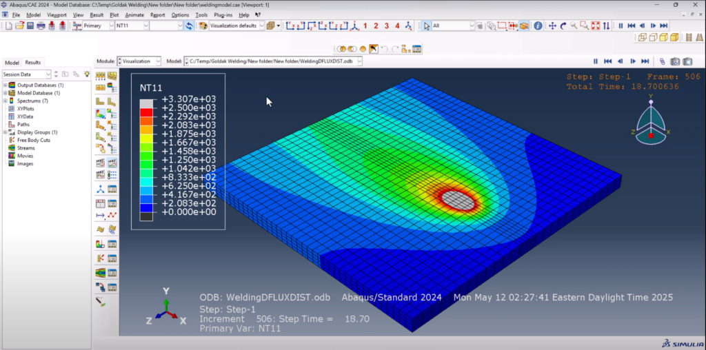
Once complete, the results are visualized in the Visualization Module:

• Contour plots show peak temperatures above 2500°C
• Animation reveals the heat source moving smoothly through the part
• By adjusting the scale (e.g., setting the max value to 2500), temperature gradients become easier to interpret

Want the Files?

📦 Skip the setup and get straight to simulation.
Download the full Goldak DFLUX model, material properties, and Fortran code below:

👉 Download the Abaqus DFLUX Welding Simulation Files

Final Thoughts

This is the most complete Abaqus Goldak DFLUX welding simulation tutorial you’ll find online. No hidden code. No skipped steps. Just a working, realistic heat source that you can reuse, tweak, or expand for your own welding studies.

If you’re doing heat transfer, welding FEA, or trying to predict thermal fields during arc welding—this method gives you complete control.

📺 Watch the tutorial on YouTube:
👉 Abaqus Goldak DFLUX Welding Simulation

💬 Found it helpful? Let me know in the comments. It’s free, and it helps me keep making content like this.

🔔 Subscribe to FEA Master for more tutorials on Abaqus, subroutines, and real-world simulation workflows.