In this in-depth Abaqus Three Point Bending XFEM Crack growth simulation, we simulate crack growth in a three-point bending test using the powerful Extended Finite Element Method (XFEM). Whether you’re exploring fracture mechanics for the first time or troubleshooting past failures, this guide walks you through the entire setup: from geometry modeling and material property definition to crack initiation, propagation, and visualizing crack evolution through post-processing fields like Status XFEM, PHILSM, and PSILSM.
Watch the video here:
Table of Contents
Creating the Geometry in Abaqus
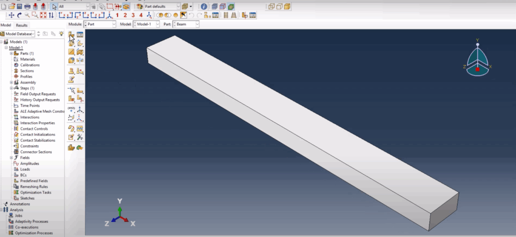
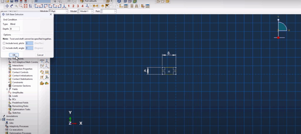
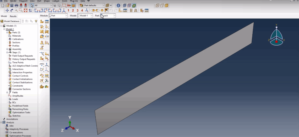
We begin by building three parts: the beam, the span (supports), and the crack. The beam is modeled as a 3D deformable solid using extrusion, with dimensions of 80 mm in length, 4 mm in height, and 8 mm in width. For the support, we create a 3D discrete rigid solid—initially solid but later converted to a shell to avoid assembly errors. This part is also extruded with dimensions of 8×4×8 mm. Lastly, the crack is modeled as a simple 1 mm line using a 3D shell extrusion, matching the depth of the beam to allow proper XFEM tracking.
Assigning Material Properties and Fracture Behavior
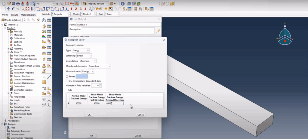
We define material properties that simulate realistic fracture behavior in the beam. The density is set to 7.8e-9, with an elastic modulus of 210,000 MPa and a Poisson’s ratio of 0.3. To simulate damage, we add traction-separation behavior with a max nominal stress of 120 MPa and damage evolution based on energy dissipation using a power-law mode. The fracture energy is defined as 40,000 J, and a stabilization value of 1e-5 is introduced for cohesive behavior to ensure convergence. Once all properties are assigned, we create a solid homogeneous section and apply it only to the beam. The span and crack do not require sections. Abaqus Three Point Bending XFEM Crack growth simulation
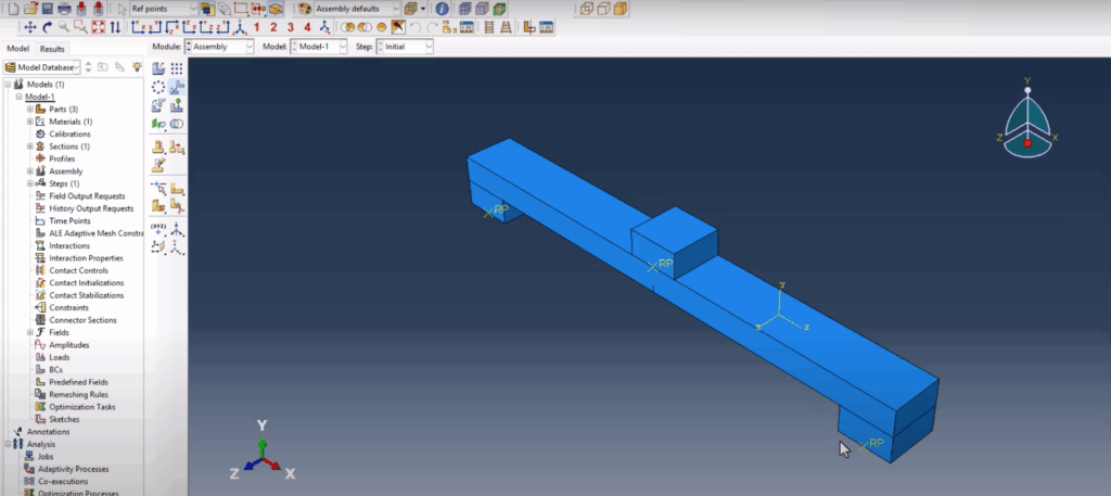
Assembly and Reference Points
After preparing the parts, we fix a typical Abaqus issue where discrete rigid solids cannot be used directly in assemblies by converting the span to a shell. Additionally, we assign reference points on the supports, enabling us to apply boundary conditions without defining rigid body constraints manually. The parts are then placed and translated into their correct positions. Multiple instances of the span are created, and the final assembly is aligned precisely to ensure mesh connectivity and load distribution. Abaqus Three Point Bending XFEM Crack growth simulation
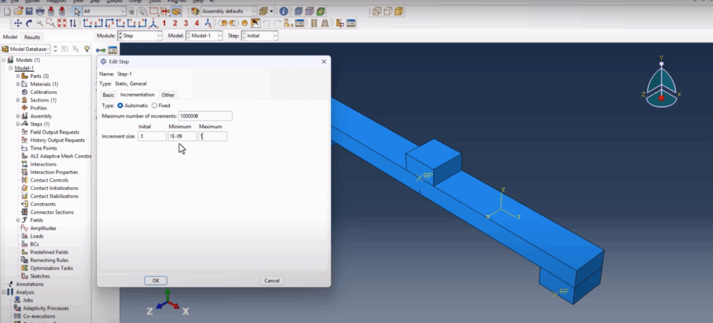
Step Creation and Output Requests
We define a static general step for the simulation with a maximum time of 1e6, initial increment of 0.1, minimum increment of 1e-9, and max increment of 1. Abaqus’s Field Output Manager is configured to record key fracture fields. We enable output for Status XFEM to track crack growth and also enable PHILSM and PSILSM, which are crucial for understanding level set field contours. These fields help in visualizing where the crack is located and how it is propagating. Abaqus Three Point Bending XFEM Crack growth simulation
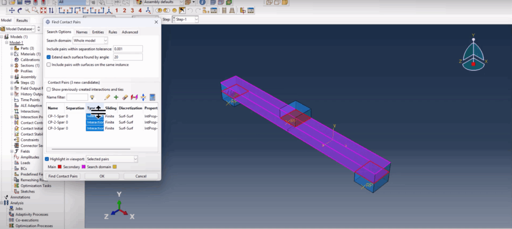
Defining Interactions and XFEM Crack Setup
To simulate realistic contact, we define interaction properties with tangential behavior using a penalty method and a friction coefficient of 0.15, along with a hard normal contact. Rather than manually selecting surfaces, we use the “Find Contact Pairs” feature to automate detection and creation of contact interactions between the beam and spans. For the crack definition, we use the special crack interaction module, select XFEM as the crack type, define the crack domain as the beam, and pick the crack part for location. Then, we activate crack growth by creating an initial XFEM crack growth interaction referencing the defined crack. Abaqus Three Point Bending XFEM Crack growth simulation
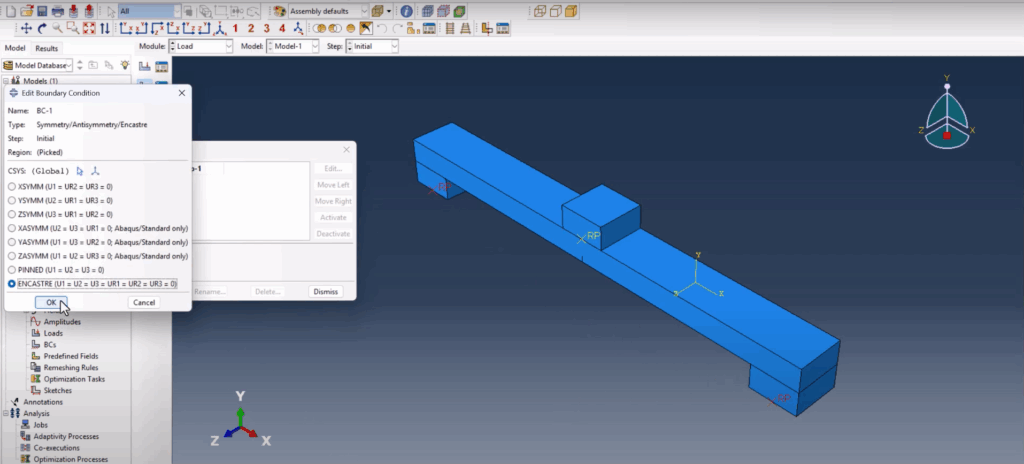
Loads and Boundary Conditions
Two boundary conditions are applied: an encastre condition (fully fixed) to both spans using their reference points, and a displacement condition of -8 mm applied downward to the top span to simulate the bending load. The negative Y-direction load simulates realistic crack initiation from the bottom center of the beam. Abaqus Three Point Bending XFEM Crack growth simulation
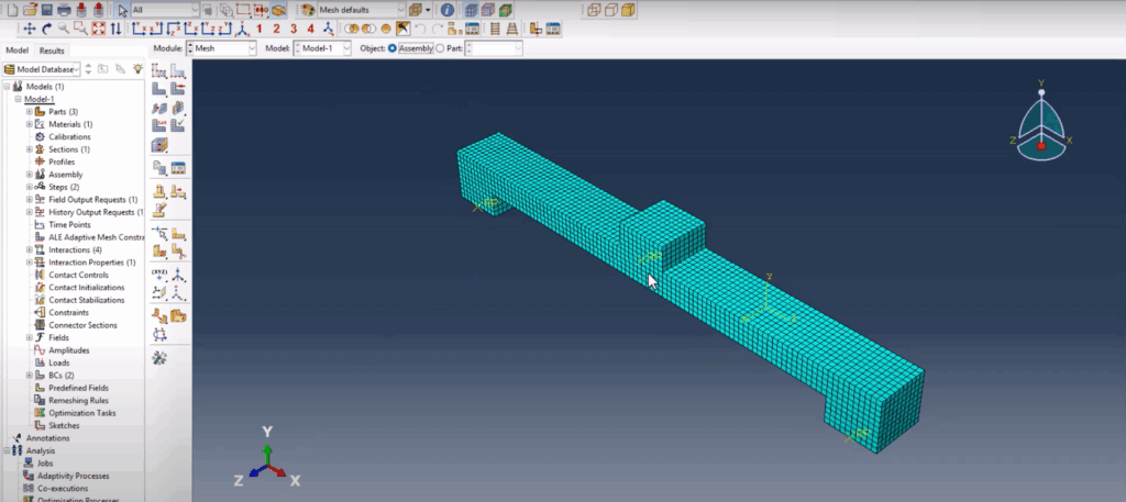
Meshing and Node Matching
Mesh quality is crucial for convergence and accuracy. The span and beam parts are meshed with a global seed size of 0.8 mm using quad-structured elements. The mesh control ensures that matching nodes are aligned at the contact interfaces, which is visually verified. A mismatch in node alignment could cause simulation errors or invalid contact behavior, so maintaining consistent seed sizes is essential. Abaqus Three Point Bending XFEM Crack growth simulation
Running the Job and Monitoring Results
We create a job named “three-point bending XFEM” and run the simulation. Abaqus may throw a warning about some parts lacking section assignment (like the rigid spans), but this is acceptable. The job runs without fatal errors, though coarse mesh or high displacements may cause it to abort depending on system limitations. However, the setup is fully educational and modifiable for your specific needs.
Abaqus Three Point Bending XFEM Crack growth simulatio Abaqus Three Point Bending XFEM Crack growth simulation
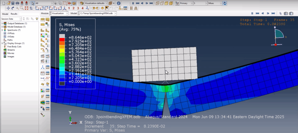
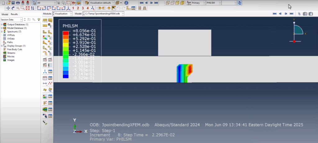
Post-Processing and Crack Visualization
The final results are explored using animations and field contours. We observe the downward movement of the top span and crack propagation from the beam center. Using the Free Edges view, the crack becomes visually distinguishable. Slow-motion animation helps track how the crack front moves upward with increasing displacement. We also inspect the PHILSM (signed distance function for crack surface) and PSILSM (crack front direction) fields. These fields allow precise tracking of the crack surface and direction. Finally, using Status XFEM, we confirm which elements are enriched (value of 1 means cracked), making it a powerful diagnostic field. Abaqus Three Point Bending XFEM Crack growth simulation
Conclusion
This tutorial demonstrates a complete XFEM-based fracture simulation for a three-point bending test in Abaqus. From geometry setup to crack propagation visualization, every step is designed to help you confidently simulate brittle fracture using XFEM. If you’re looking to expand into fatigue or weld cracking simulations, this is the perfect foundation to build on. Abaqus Three Point Bending XFEM Crack growth simulation
📺 Watch the full step-by-step simulation video now
Abaqus Three Point Bending XFEM Crack growth simulation
🔥 Want to learn welding simulation in Abaqus next? Check this one:
https://feamaster.com/abaqus-goldak-dflux-welding-simulation
Abaqus Three Point Bending XFEM Crack growth simulationAbaqus Three Point Bending XFEM Crack growth simulationAbaqus Three Point Bending XFEM Crack growth simulationAbaqus Three Point Bending XFEM Crack growth simulation
