Welding residual stress Abaqus simulations can be much simpler than you think. In this tutorial, you’ll learn how to predict residual stress without coding, using only thermal results from a previous simulation.
This is the best method I’ve found to simulate welding residual stress in Abaqus, and it’s far simpler than you might expect.
Ready? Let’s get into it.
🔗 Watch the full video tutorial here:
Step 1: Use a Thermal Welding Distribution File
In this tutorial, I’m using a welding distribution file generated from a previous simulation. If you haven’t seen that video yet, I highly recommend watching it first—it explains how the heat distribution was created step by step. You can find it here: Watch the welding simulation video. If you’d rather skip the simulation setup and jump straight into the residual stress analysis, you can download the complete simulation package—CAE and ODB files included—from the official site: Download the welding simulation files from FEAMaster.com.
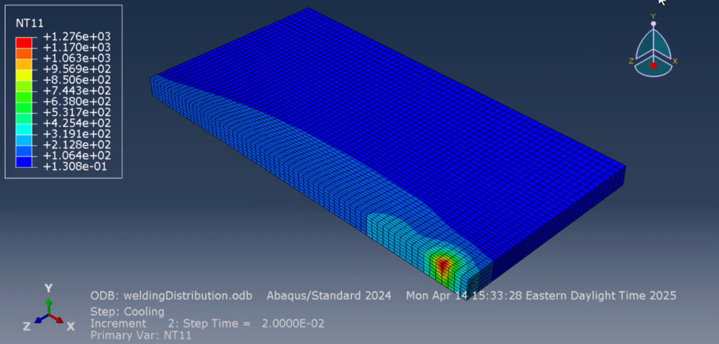
When I run the animation of the original welding simulation, you’ll see the heat flux passes through the plate and reaches room temperature. The highest temperature stabilizes, and that ODB file will be used for residual stress calculation.
Step 2: Duplicate the Model and Set Up the New Residual Stress Simulation
Open the original CAE file. This is the model we used for thermal simulation. First, duplicate the model and rename it to something like residual_stress. You’ll notice the underline beneath the model name helps you verify which model you’re in.
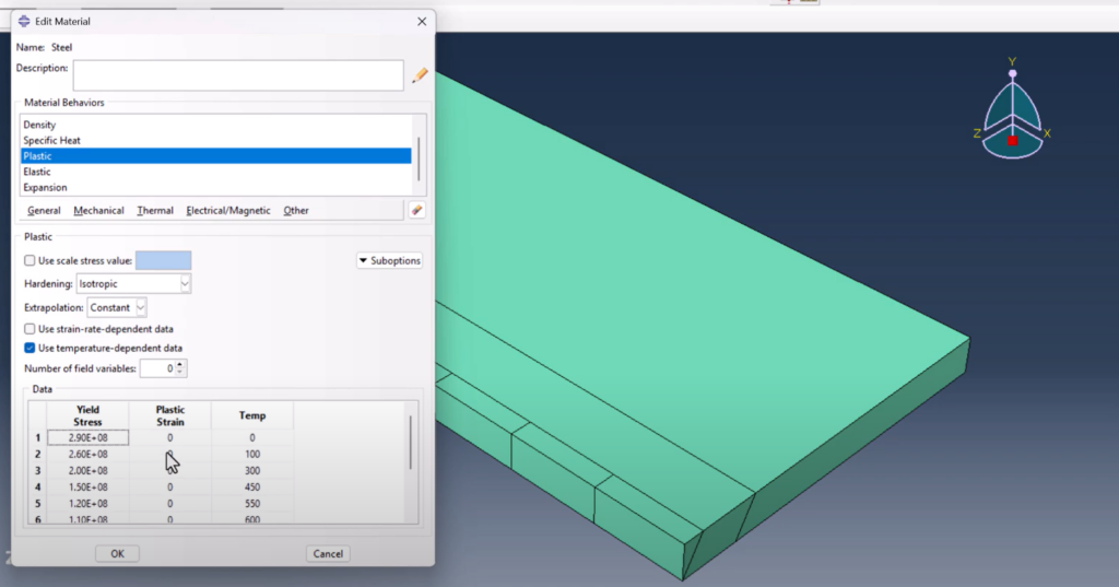
Let’s open the material properties. In the original model, we only had temperature-based properties like conductivity and specific heat. But for mechanical analysis, we now need to define:
Elasticity (temperature-dependent)
Plasticity (perfectly plastic assumption)
Thermal expansion (again, temperature-dependent)
To make this easier, I’ve provided a free Excel file with temperature-dependent material data. You can download it from here under the “Material Properties Package”—just add it to your cart and download it after checkout.
Copy and paste the values for elastic modulus, plasticity (strain = 0, perfectly plastic), and expansion directly from the spreadsheet into your material definition in Abaqus. That’s it for materials.
Step 3: Create a New Static General Step
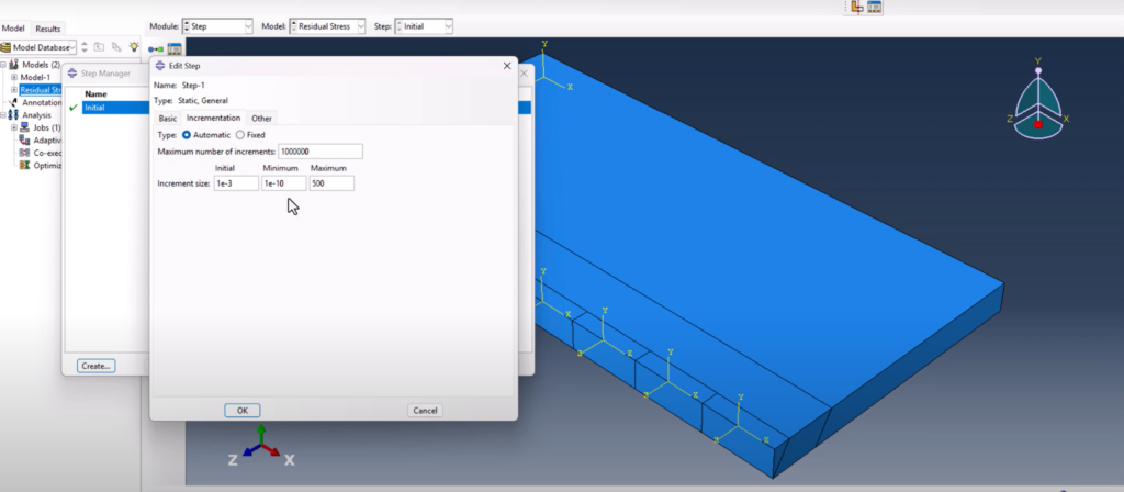
Go to the step manager and delete all the thermal steps. Select the first one, hold shift, and delete through the last. Now create a Static General step.
Since the cooling duration in our previous model was 2000 seconds, I’ll use a similar value—2025 seconds to keep it in context for the year. Set the time increment to 1e-3, with minimum and maximum of 1e-10 and 500 respectively.
Next, edit the field output. Remove all unnecessary variables and retain only the stress components. This keeps the ODB file lightweight and easy to analyze.
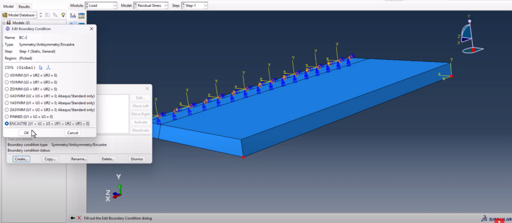
Step 4: Apply Symmetry and Encastre Boundary Conditions
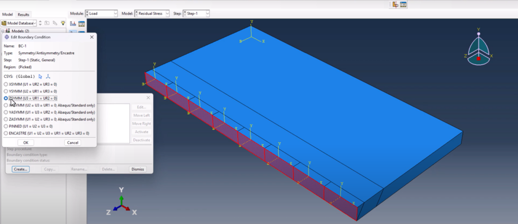
We’re using a symmetric model, so symmetry boundary conditions are essential. Apply Z-symmetry on the appropriate surfaces. Then rotate the model to locate the nodes where constraints are needed.
Select two edge nodes using shift-click and apply an encastre boundary condition. This simulates real-world constraints like clamps or spot welds applied during the actual welding process.
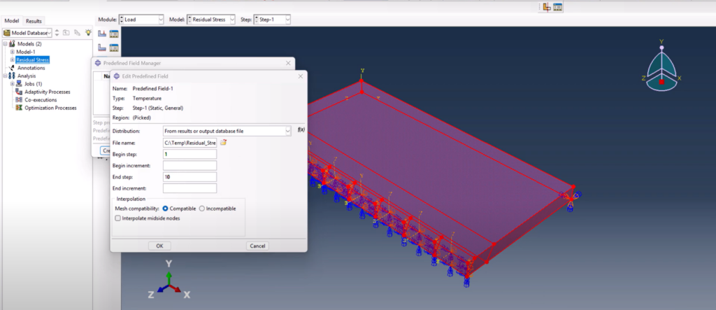
Step 5: Map Temperature Results From the Welding Simulation
Head over to the Predefined Field Manager and create a new temperature field. Select the whole model and choose “From Output File” instead of direct specification. Browse and load the previous ODB file.
Set the starting step to 1 and ending step to 10—this captures the full cooling period. With this step, you’re now coupling the thermal results directly with your mechanical model, enabling residual stress prediction.
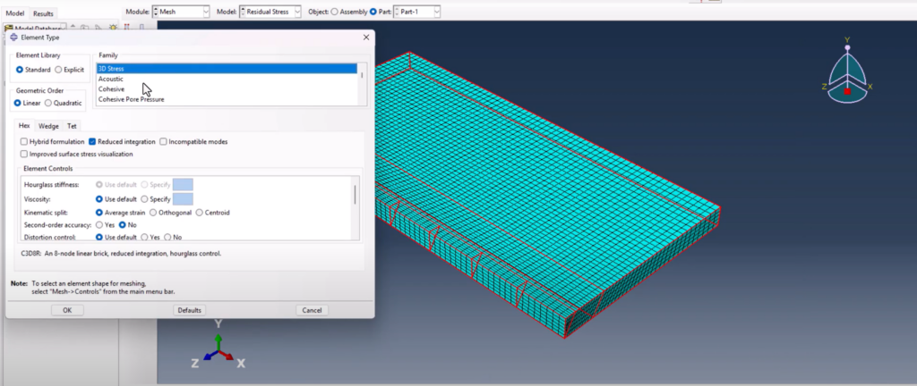
Step 6: Update Mesh Type for Stress Analysis
Go to the mesh module and convert your part to 3D stress elements. Previously it was set for heat transfer. Switch to C3D8R or appropriate stress-compatible elements and regenerate the mesh.
Step 7: Create and Run the Job
Before we start the job, a small favor—if this walkthrough helped you so far, leave a comment on the video. It’s free, and your support helps me grow and keep making quality tutorials like this.
Now, go to the Job Manager and create a new job named residual_stress. Under parallelization, choose 8 CPUs if your system supports it—this will speed up the job.
Submit the job. You may see some warnings; ignore them unless they escalate into errors. Let the simulation run, and once it’s complete, we’ll review the results.
Step 8: Analyze and Validate the Residual Stress Results
With the simulation complete, open the result file. Run an animation first to visualize stress evolution during cooling.
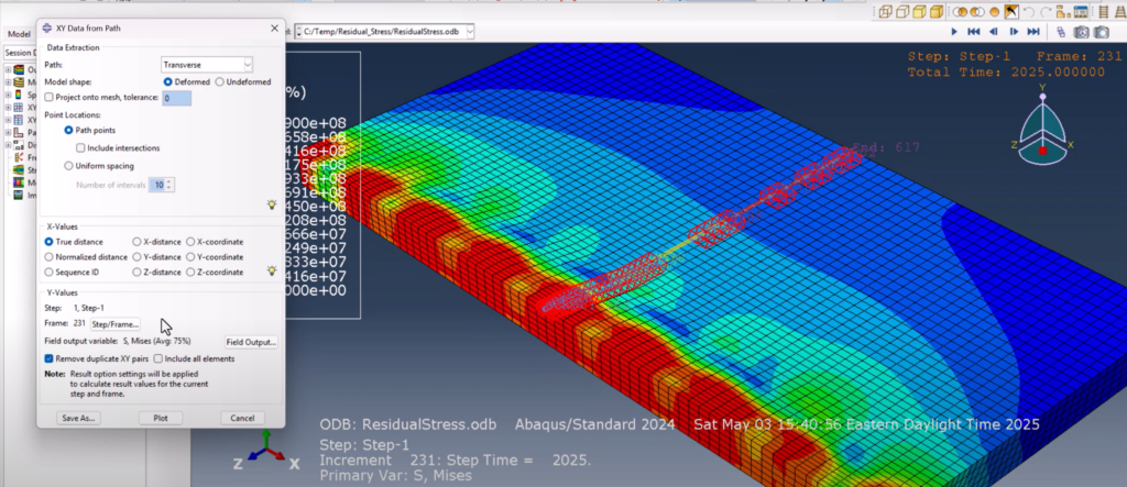
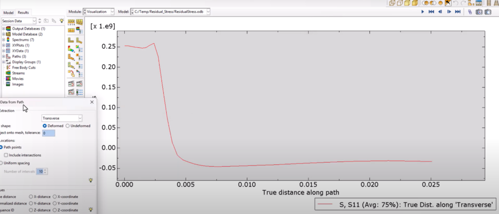
You can now plot residual stress paths. From Tools > Path, create a transverse path by selecting nodes across the weld zone. I already created a path earlier to save time.
In XY Data, use the path to plot variables like:
Von Mises stress
S11 (longitudinal stress)
S33 (through-thickness stress)
The Von Mises plot should show a classic weld profile—high in the HAZ, tapering outwards. When compared with academic literature or experimental data, it aligns well, indicating the model is physically realistic.
Final Words
This no-coding method gives you a fast, accessible, and surprisingly accurate way to simulate welding residual stress in Abaqus. You reuse temperature history from a previous simulation, apply basic material properties, and use predefined temperature fields to drive the stress analysis. That’s it.
✅ No DFLUX. ✅ No USDFLD. ✅ No subroutines. Just smart use of Abaqus’ built-in capabilities.
If you want to go even further and simulate welding using DFLUX, check out the next video linked on screen. It’s a step-by-step breakdown of how to create a moving heat source in Abaqus for welding analysis.