Performing a Welding Simulation in Abaqus Without DFLUX dramatically simplifies the modeling workflow, removes the need for Fortran subroutines, and accelerates your simulation setup.
This detailed guide walks you through exactly how to simulate welding heat transfer and residual stress inside Abaqus CAE — using only standard tools — without any coding or subroutine integration. Watch this video to learn how to model welding simulation in Abaqus without the subroutine of DFLUX:
Creating the Geometry and Partitioning for Welding Simulation
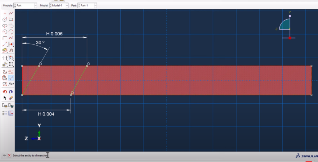
Starting with the geometry, we create a simple rectangular solid representing a metal plate. Using the Part module, a 3D deformable solid is sketched and extruded to dimensions approximately 50 mm in length, 5 mm in width, and 0.2 mm in thickness.
To realistically model welding, partitions are made carefully. A bevel cut is created by sketching a 30-degree angled line, separating the weld material from the base metal.
Further partitioning divides the structure into distinct zones: the weld, the immediate heat-affected zone (HAZ), and the base material.
Symmetry is implemented along the midplane of the plate to reduce computational cost while maintaining physical realism.
Assigning Temperature-Dependent Material Properties
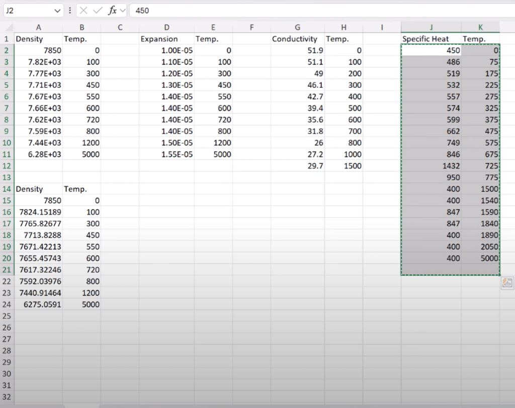
Material properties are assigned next. In the Property module, a new material representing steel is defined.
Temperature-dependent thermal conductivity, specific heat, density, and elastic modulus values are inputted.
A solid homogeneous section is created and assigned to the entire part.
Sets are carefully created for the weld zone, the HAZ, and the base material to simplify later load and boundary condition applications.
Meshing Strategy for Accurate Welding Simulation
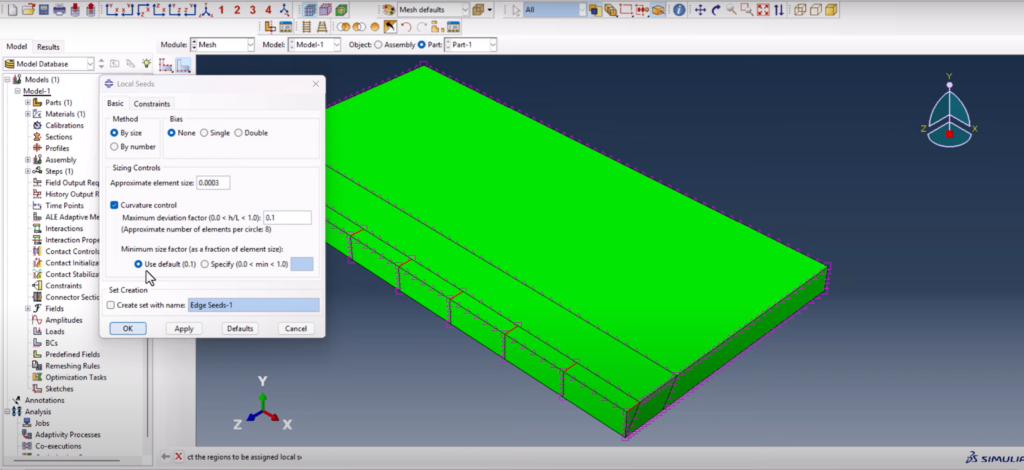
Meshing is handled with special attention near the weld line. Mesh seeds are defined using biasing: finer elements near the weld zone and gradually coarser elements farther from it.
The sweep meshing technique is used to maintain structured, high-quality elements across partitions.
This refined mesh ensures sharp thermal gradients during welding and cooling are accurately captured.
Assembly and Interaction Setup
The part is positioned correctly in the Assembly module.
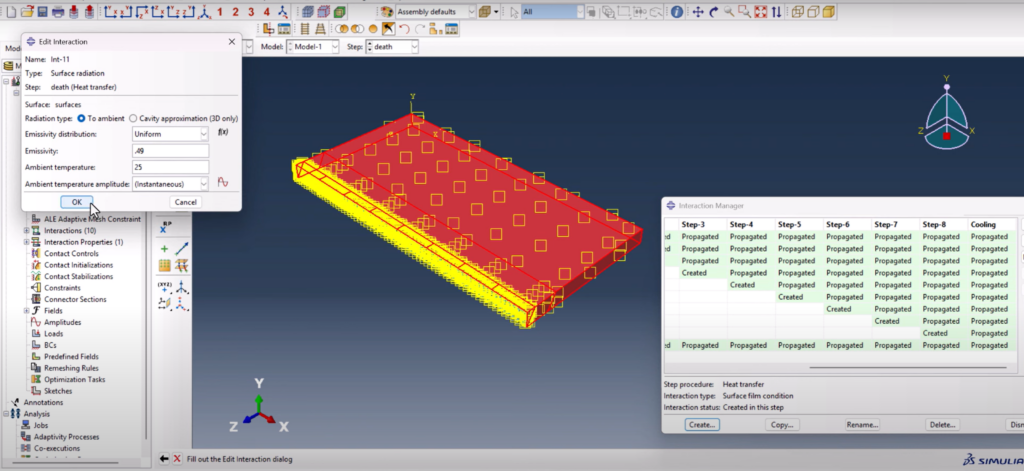
Surface interactions are then assigned to model environmental effects:
- A Surface Film Condition simulates convective heat transfer with the ambient environment.
- Radiation to Ambient interactions simulate radiative heat loss, completing a realistic boundary environment.
Both interactions are critical for accurate cooling simulation post-welding.
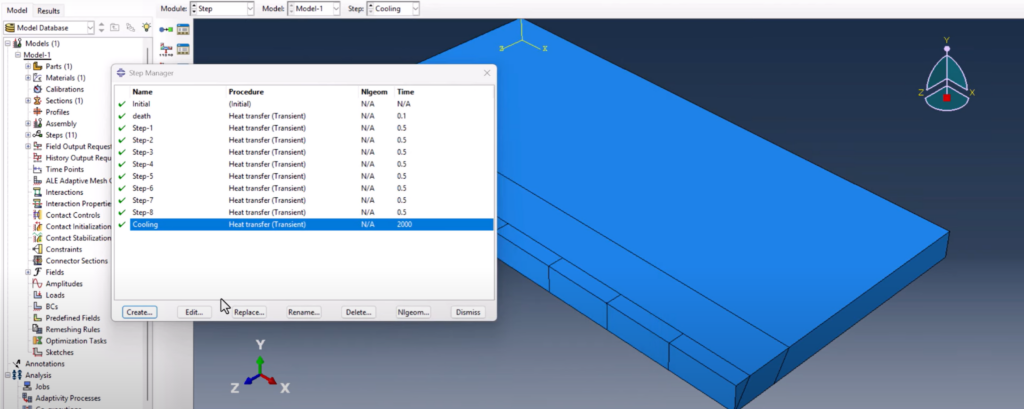
Step Definitions for Welding Simulation in Abaqus Without DFLUX
The analysis steps are carefully designed:
- Initial Step: Establish baseline conditions.
- Welding Phase Step: Apply transient heat flux to the weld zone.
- Cooling Phase Step: Model natural cooling after welding stops.
- Static General Step: Calculate residual stresses after cooling.
Time increments are adjusted for each phase to balance accuracy and computational efficiency.
Applying Heat Flux Without DFLUX Subroutine
Instead of writing a DFLUX subroutine, the heat flux is applied statically and directly onto the weld zone.
Heat input is calculated based on process parameters (22 V, 57 A, 12.5 mm/s speed, and 0.65 efficiency) to achieve approximately 75.35 J/mm.
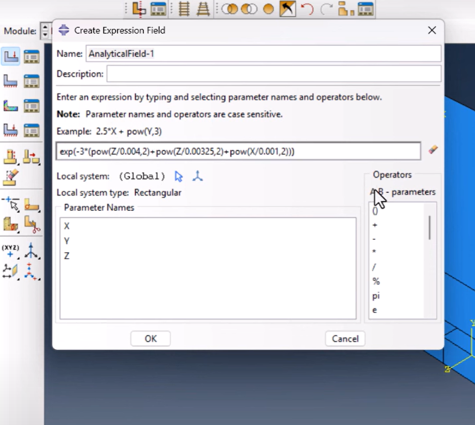
An Analytical Field in Abaqus distributes this heat flux realistically across the weld surface during the welding step. In the video I mistakenly repeated the Z terms earlier. The correct form of the equation is: exp(-3 * (pow(Y/0.004, 2) + pow(Z/0.00325, 2) + pow(X/0.001, 2)))
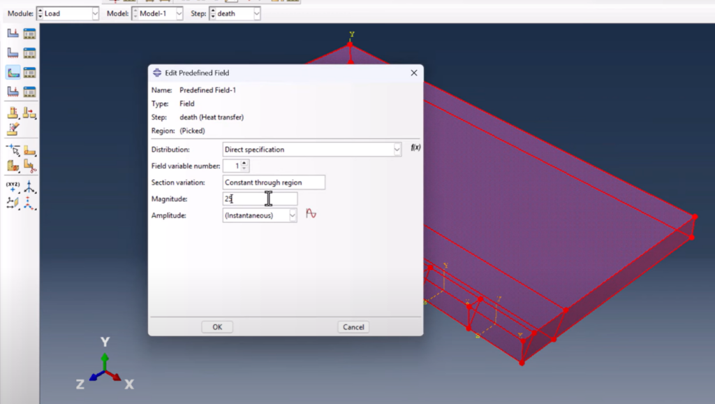
Defining Boundary Conditions and Mechanical Constraints
Initial temperature conditions are set at 25°C uniformly.
Symmetry boundary conditions are applied along the partitioned midplane.
One node is fixed in all directions to prevent rigid body motion while still allowing thermal expansion and contraction.
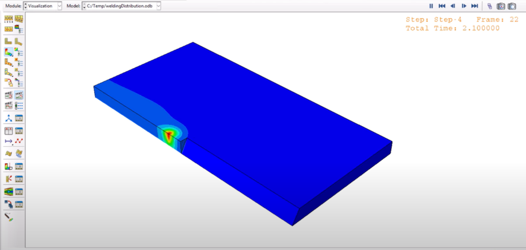
Running the Simulation and Post-Processing Results
The job is created and submitted with all defined steps, interactions, and loads.
Temperature distributions are tracked during welding and cooling.
Residual stress fields are analyzed after cooling is complete.
Temperature-time histories are extracted at critical points for validation.
Mesh sensitivity studies are optionally performed to confirm result stability.
Benefits of Welding Simulation in Abaqus Without DFLUX
Choosing to perform a Welding Simulation in Abaqus Without DFLUX eliminates dependency on custom Fortran code, significantly reduces simulation complexity, and accelerates the setup process.
It also improves result reproducibility across multiple projects and geometries, particularly useful for structural and manufacturing simulations.
Conclusion on Using Abaqus With or Without DFLUX
Speaking from experience, using DFLUX is way easier and faster than this method. On the other hand, using coding and DFLUX would add the complexity to the project then you would have to code and debug; plus linking the Abaqus and Fortran sometimes is a pretty hard job to do. I’ll leave you to decide :).
Watch the related video on YouTube.
Enhanced Welding Simulation in Abaqus
If you want to start using subroutine, you have to try linking Abaqus with Fortran so check this blog:
#Welding #Abaqus #Nosubroutine #DFLUX
