Wire Arc Additive Manufacturing Simulation Abaqus Using Goldak DFLUX

Focus Keyword: Wire Arc Additive Manufacturing Simulation Abaqus

If you’re looking to simulate wire arc additive manufacturing Abaqus using a Goldak heat source with the DFLUX subroutine, you’ve come to the right place.

In this comprehensive tutorial, we’ll walk through every step of setting up a wire arc additive manufacturing (WAAM) simulation—from geometry modeling and meshing to defining the Goldak heat input via DFLUX and visualizing thermal history. This guide is perfect for graduate students, researchers, and engineers aiming to simulate complex heat transfer in metallic additive manufacturing processes using finite element tools.

You can watch the full video tutorial here:

Want to skip the setup and just get the working files?
👉 Download the Wire Arc Additive Manufacturing Abaqus Files

Introduction to Wire Arc Additive Manufacturing in Abaqus

Wire Arc Additive Manufacturing (WAAM) is a powerful technique used to build metal structures by feeding a wire into an electric arc. In simulation environments like Abaqus, modeling this process demands accurate thermal input, dynamic meshing, and subroutine customization.

To capture the moving heat source, the Goldak double ellipsoid model is implemented using the DFLUX subroutine. This setup simulates the temperature distribution and thermal gradients accurately as the molten pool progresses along the predefined path.

In this Wire Arc Additive Manufacturing Simulation Abaqus tutorial, we rely on a clean mesh, proper thermal boundary conditions, and a custom Fortran subroutine to simulate real-time heat input.

Step-by-Step Model Setup in Abaqus

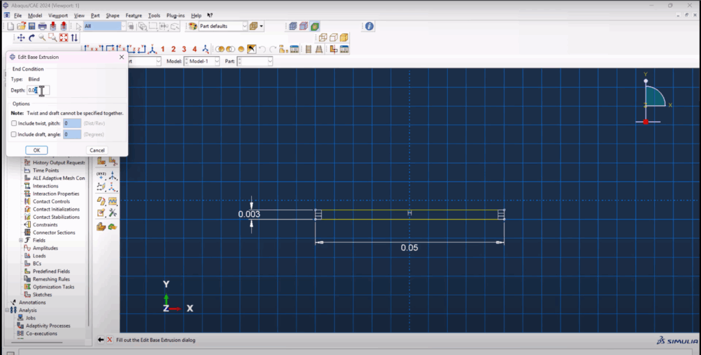
The Wire Arc Additive Manufacturing Simulation Abaqus simulation begins by creating two parts: the substrate and the deposited layer. These are modeled as 3D deformable solids.

The dimensions are small and represent a thin strip:

Substrate: 0.0025 m × 0.05 m
Layer: 0.002 m × 0.05 m × 0.004 m (height)

After extrusion, partitioning is used to define heat input paths on the substrate’s top surface. These partitions are crucial for applying the body heat flux via DFLUX.

Defining Temperature-Dependent Material Properties

Instead of using constant properties, we use temperature-dependent thermal conductivity for thi Wire Arc Additive Manufacturing Simulation Abaqus, specific heat, and density for steel. These are directly downloaded from the FEA Master material pack, and inserted into Abaqus using Excel copy-paste.

These properties are crucial for capturing:

Thermal lag and diffusion
Realistic gradients in heat-affected zones (HAZ)

Sections are created and assigned for both the substrate and the deposited layer, using the same steel material.

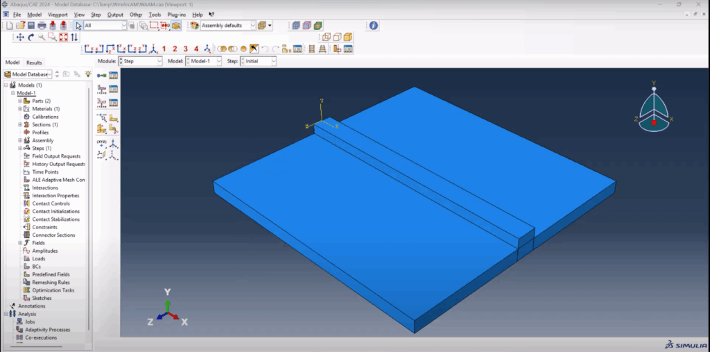
Assembly and Boundary Setup

The layer is placed directly on top of the substrate in the assembly module, and everything is defined as part-dependent to allow separate meshing.

To make the DFLUX input cleaner, the entire model is translated so the heat source starts at (0,0,0).

A tie constraint is created to thermally bind the layer to the substrate. This ensures that thermal flux transfers realistically between them, enabling temperature gradients in the substrate due to heat conduction from the layer.

Heat Transfer Step and Initial Conditions

The Wire Arc Additive Manufacturing Simulation Abaqus simulation uses a heat transfer step with:

Time period = 25 s
Initial increment = 0.1 s
Minimum increment = 1e-10
Maximum increment = 1 s
Maximum temperature = 3500°C

Mass scaling is not necessary here since it’s not a dynamic problem. A field output is customized to only capture nodal temperatures, reducing output size.

Initial temperature is defined as 25°C (predefined field), and absolute zero is set to -273.15°C.

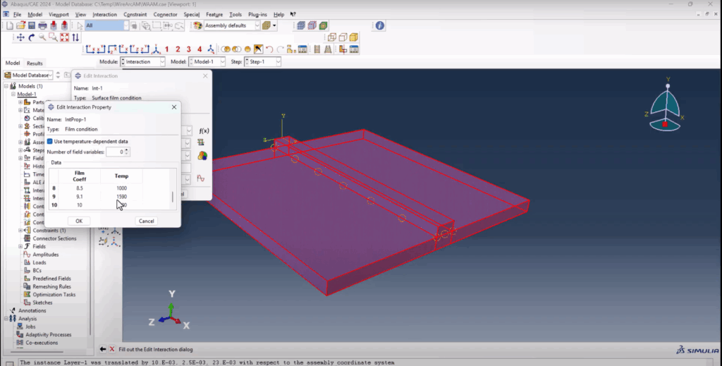
Surface Interactions: Film and Radiation

Two key thermal boundary conditions are applied:

Surface film condition using air properties (temperature-dependent h-values).
Surface radiation with an emissivity of 0.49.

These allow the part to lose heat to the environment realistically, capturing cooling effects.

Goldak DFLUX For Wire Arc Additive Manufacturing Simulation Abaqus

The main feature of this tutorial is the Goldak DFLUX subroutine for Wire Arc Additive Manufacturing Simulation Abaqus.

Key characteristics:

Implemented in Intel Fortran via Visual Studio
Uses double ellipsoid model equations
Allows dynamic front and rear heat distribution (Qf and Qr)
Heat center moves via XC = X0 + V * T

Abaqus is linked to the .for file through job settings. Users can customize the parameters:

A, Bf, Br, C (ellipsoid dimensions)
Qf, Qr (heat input)
Welding speed (V)

The subroutine was copied directly from the official Abaqus documentation and modified with custom heat source geometry and parameter tuning.

    SUBROUTINE DFLUX(FLUX,SOL,KSTEP,KINC,TIME,NOEL,NPT,COORDS,
     1 JLTYP,TEMP,PRESS,SNAME)
C
      INCLUDE 'ABA_PARAM.INC'
      DIMENSION FLUX(2), TIME(2), COORDS(3)
      CHARACTER*80 SNAME

C     Coordinates
      X = COORDS(1)
      Y = COORDS(2)
      Z = COORDS(3)

C     Heat source center (moving in X with time)
      XC = 0.0 + 0.002 * TIME(2)
      YC = 0.0D0
      ZC = 0.0D0

C     Goldak parameters (in meters)
      a  = 6  / 1000.0
      c  = 5  / 1000.0
      bf = 3.46 / 1000.0
      br = 8 / 1000.0
      ff = 0.57D0
      fr = 1.43D0
      PI = 3.1415D0

C     Heat input parameters
      eta = 0.8
      V   = 23.0
      I   = 232.0
      Q   = eta * V * I

      Qr = (6.0D0 * Q * fr) / (a * br * c * PI * SQRT(PI))
      Qf = (6.0D0 * Q * ff) / (a * bf * c * PI * SQRT(PI))

C     Rear half (X <= XC)
      IF (X .LE. XC) THEN
         IF ( (((X - XC)**2) / (a**2)) + (((Y - YC)**2) / (br**2)) +
     &        (((Z - ZC)**2) / (c**2)) .LT. 1.0D0 ) THEN

            FLUX(1) = Qr * EXP( -3.0D0 * ( ((X - XC)**2) / (a**2) +
     &                                   ((Y - YC)**2) / (br**2) +
     &                                   ((Z - ZC)**2) / (c**2) ) )
         ENDIF

C     Front half (X > XC)
      ELSEIF (X .GT. XC) THEN
         IF ( (((X - XC)**2) / (a**2)) + (((Y - YC)**2) / (bf**2)) +
     &        (((Z - ZC)**2) / (c**2)) .LT. 1.0D0 ) THEN

            FLUX(1) = Qf * EXP( -3.0D0 * ( ((X - XC)**2) / (a**2) +
     &                                   ((Y - YC)**2) / (bf**2) +
     &                                   ((Z - ZC)**2) / (c**2) ) )
         ENDIF
      ENDIF

      FLUX(2) = 0.0D0

      RETURN
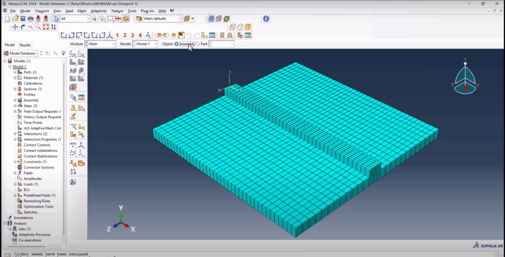
      END

Mesh Refinement and Compatibility

Mesh density is carefully controlled:

40 elements along the weld path
6–8 elements through the thickness

This ensures enough resolution for temperature gradients without overloading the solver. Structured meshing is used wherever possible, and element type is assigned as DC3D8 (heat transfer brick).

Matching edge lines are validated in the assembly to ensure proper heat propagation between the layer and substrate.

Postprocessing and Thermal Analysis

After submitting the job, results are visualized in the Visualization module.

Temperature distribution is tracked via animation, showing the movement of the heat source along the path.

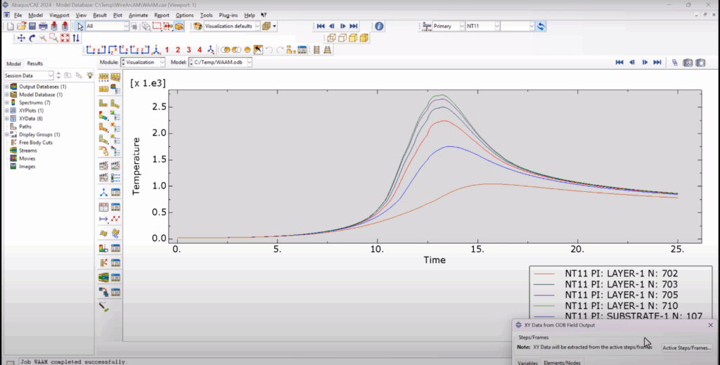
To extract thermal history:

Select multiple nodes along the build height
Use XY data → ODB Field Output
Export temperature vs. time plots

You can copy the results into Excel to customize your plots. This provides real-time insights into how temperatures evolve during the build.

For better viewing, feature edges are enabled, and cross-sectional cuts are applied.

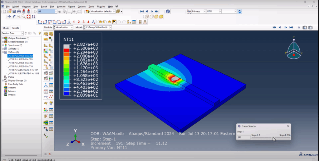
Wire Arc Additive Manufacturing Simulation Abaqus

Download the Files or Skip the Setup

🎯 Want to skip the modeling and go straight to simulation?

Get the full model and subroutine files from the official product page:
👉 Download the Abaqus DFLUX Welding Simulation Package

Final Thoughts

This wire arc additive manufacturing simulation in Abaqus provides a practical, hands-on example of thermal modeling using a moving heat source. Whether you’re building models for your thesis, academic research, or industrial testing, this setup offers a proven and clean structure to replicate and build upon.

Make sure to check out the full tutorial video for visual guidance:
▶️ Watch on YouTube

If this helped, please like the video and share the post. Got questions? Drop them in the comments—let’s build the future of simulation together!